What is Phasor Diagram?
Phasor diagram of Simple Harmonic Motion is a graphical representation of position ( i.e. phase ) of particles having same frequency but in different phase angles and amplitudes.
Using a phasor diagram, it becomes easy to analyze situations of simple harmonic motions. To draw the phasor diagram, we proceed as follows –
- It is a custom to assume that the initial position of particle is at mean position i.e. when ( t = 0 ) , position of particle is at ( x = 0 )
- Particle is moving in clockwise direction in with uniform circular motion.
- General form of simple harmonic motion equation is then taken as –
x = A \sin ( \omega t + \phi _ { 0 } )
Problem solving using Phasor diagram
Using phasor diagram, solution of numerical problems become easier as illustrated in following examples –
EXAMPLE – 1
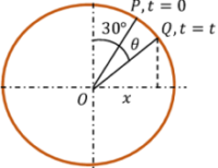
Consider about the phasor diagram of a particle moving with uniform circular motion as shown in figure. We have to find the general equation of motion.
From the geometry of given phasor diagram, we have –
\phi _ { 0 } = 30 \degree = \left ( \frac { \pi }{ 6 } \right )
Therefore, general equation of the motion of particle will be –
x = - A \sin ( \omega t + \phi _ { 0 } )
Or, \quad x = - A \sin \left [ \omega t + \left ( \frac { \pi }{ 6 } \right ) \right ]
EXAMPLE – 2
The initial position of a particle is at \left ( x = + \frac{ A }{ 2 } \right ) and it is moving in positive ( x ) direction. Determine the general equation of motion.
Phasor diagram for the motion of particle is drawn as shown in figure. Suppose that, the particle is moving in clockwise direction on a circular path.
Given, the particle is initially at \left ( x = + \frac{ A }{ 2 } \right ) . Then, the position of particle may be either at P or Q .
But, particle is moving in positive ( x ) direction. This means that, the particle is moving from \left ( x = \frac {A}{2} \right ) to ( x = + A ) . Hence, it become clear that the particle is initially at position P . The phasor diagram is now completed.
From phasor diagram, we will get –
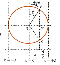
\left [ \frac { \left ( \frac { A }{ 2 } \right ) }{ A } \right ] = \cos \angle { POP' } = \left ( \frac { 1 }{ 2 } \right )
Or, \quad \angle { POP' } = 60 \degree
Therefore, \quad \phi = \left ( 90 - 60 \right ) \degree = \left ( \frac { \pi }{ 6 } \right )
Hence, simple harmonic motion equation for the particle will be –
x = A \sin \left [ \omega t + \left ( \frac { \pi }{ 6 } \right ) \right ]
Phase
In simple harmonic motion, phase of a particle is defined as the angular displacement ( in radians ) subtended at an instant reckoned from a reference point.
In simple harmonic motion, velocity of particle is zero when displacement is maximum i.e. at extreme position. Also, velocity is maximum when the particle is at its mean position i.e. when displacement is zero.
This means that –
Maximum velocity of the particle had completed at \left ( \frac {\pi}{2} \right ) radians earlier of the instance of maximum displacement.
Therefore, if we plot displacement and velocity on a graph, velocity curve will be leading by \left ( \frac {\pi}{2} \right ) radians from the displacement curve. This situation is expressed by the term phase.
Thus, phase of velocity curve is \left ( \frac {\pi}{2} \right ) radians in advance of displacement curve.
Phase Angle
Consider about a particle in simple harmonic motion. Let, the particle is at extreme position ( x = +A ) at time ( t = 0 ) . Then its equations will be –
Displacement equation \quad x = A \cos \omega t . Velocity equation \quad v = \left ( \frac { d x }{ d t } \right ) = - \omega A \sin \omega t
Or, \quad v = \omega A \cos \left ( \omega t + \frac { \pi }{ 2 } \right )
Acceleration equation \quad a = \left ( \frac { d v }{ d t } \right ) = - \omega ^2 A \cos \omega t
Or, \quad a = \omega ^2 A \cos ( \omega t + \pi )
In above equations, term ( \omega t ) is called phase angle.
From definition of time period of a simple harmonic motion, we have –
T = \left ( \frac { 2 \pi }{ \omega } \right )
Therefore, phase angle at any instant ( t = t ) is given by –
\omega t = \left ( \frac { 2 \pi }{ T } \right ) t
So, \quad \text {Phase angle} = \text {Time} \times \left ( \frac { 2 \pi }{\text {Time period}} \right )
Phase relationship in Simple Harmonic Motion
To understand the characteristics of simple harmonic motion, we can find the values of ( x, \ v, \ \text {and} \ a ) at various instants of time in one complete cycle. These values are then tabulated below –
| Time ( t ) | ( 0 ), \ ( T ) | \left ( \frac { T }{ 4 } \right ) | \left ( \frac { T }{ 2 } \right ) | \left ( \frac { 3T }{ 4 } \right ) |
| Phase angle ( \omega t ) | ( 0 ), \ ( 2 \pi ) | \left ( \frac { \pi }{ 2 } \right ) | ( \pi ) | \left ( \frac { 3 \pi }{ 2 } \right ) |
| Displacement ( x ) | ( + A ) | ( 0 ) | ( - A ) | ( 0 ) |
| Velocity ( v ) | ( 0 ) | \left ( - \omega A \right ) | ( 0 ) | ( + \omega A ) |
| Acceleration ( a ) | ( - \omega ^2 A ) | ( 0 ) | ( + \omega ^2 A ) | ( 0 ) |
These values are plotted on a graph as shown in following figures. It is called phase relationship diagram of simple harmonic motion.
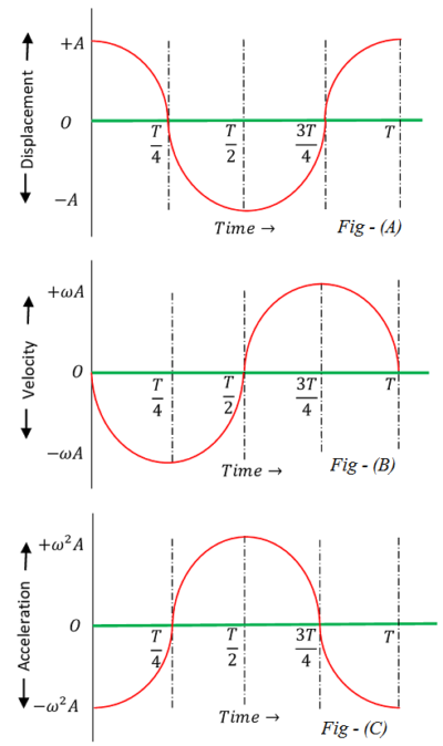
- Fig (A) shows plotting of linear displacement with respect to time.
- Fig (B) shows variation of linear velocity with respect to time.
- Fig (C) shows variation of linear acceleration with respect to time.
Properties of Simple Harmonic Motion
Properties of simple harmonic motion can be narrated from phase relationship diagram.
These properties are –
- Displacement, velocity and acceleration all are varying harmonically with respect to time.
- Maximum velocity is ( \omega ) times of displacement amplitude ( A ) .
- Maximum acceleration is ( \omega ^2 ) times of displacement amplitude ( A ) .
- Phase of velocity curve is \left ( \frac {T}{4} \right ) or \left ( \frac {\pi}{2} \right ) radians ahead of displacement curve. This means that at an instant, when displacement achieves maximum value, the velocity has completed its maximum value at \left ( \frac {\pi}{2} \right ) radians earlier of that instant.
- Thus phase difference between velocity curve and displacement curve is \left ( \frac {\pi}{2} \right ) .
- When displacement is zero velocity is maximum and vice versa.
- Phase of acceleration curve is \left ( \frac {T}{2} \right ) or \left ( \pi \right ) radians ahead of displacement curve. This means that, at an instant when displacement has achieved maximum value, the acceleration has completed its maximum value at \left ( \pi \right ) radians earlier of that instant.
- Therefore, acceleration curve is leading by \left ( \pi \right ) radians from the displacement curve. Thus phase difference between acceleration curve and displacement curve is \left ( \pi \right ) .
- When displacement is zero, acceleration is also zero.
See numerical problems based on this article.