Alternating Current

What is an Alternating Current?

An electric current in which the magnitude of current and polarity both changes periodically with time is called an Alternating Current (AC)

Most of electric appliances run on alternating current.
Electric supply for domestic, commercial and industrial use are mainly AC in nature.

Advantages of AC over DC supply

AC supply has advantages over DC supply as –

Generation, transmission and distribution of AC is more economical due to less expensive as compared to that of DC.
The alternating voltage can be step down or step up easily using a transformer.
AC travels on the surface of a conductor, so costly conducting materials can be saved for long transmission by using inner core of cheaper material say steel e.g. ACSR (i.e. aluminium conductor steel reinforced) is widely used for electric supply lines.
AC can reach distant places with reduced loss of electric power (by using a transformer).
Alternating voltage can be better controlled without any loss of electric power (say by using a choke coil).
AC is easily converted into DC by using rectifiers.
AC machines are smaller in size, having longer life and easy to use.

Disadvantages of AC over DC supply

AC supply has some disadvantages over DC supply as –

AC can be more harmful than DC of same intensity. This is because maximum value or peak value of AC is $( \sqrt {2} )$ times that of the effective value. For example – well known domestic supply of $( 220 \ V \ AC )$ has a peak value given by $[( \sqrt {2} \times 220 \ V ) = 311 \ V ]$ and harm more as compared to $( 220 \ V \ DC )$ .
AC cannot be used in electrolysis processes such as electroplating, electrotyping and electrorefining, where only DC is used.
AC in a wire is not uniformly distributed throughout its cross-section. The current density is much greater on the surface of the wire than that inside the wire. This concentration of AC near the surface of the wire is called skin effect. Therefore, inner conducting material of the transmission wire remains unused.

Peak value of an AC Current

If an AC supply is viewed on an oscilloscope, it will look like a sine or cosine wave as shown in figure.

A sinusoidal alternating current is expressed as –

$I = I_0 \sin ( \omega t )$ ……… (1)

Here, $( I_0 )$ is called as –

The Maximum value or Peak value of alternating current or
Amplitude of alternating current.

The angular velocity $( \omega )$ of alternating current is given by –

$\omega = \left ( \frac {2 \pi}{T} \right ) = 2 \pi \nu$ .

Here $( T )$ is the time period and $( \nu )$ is the frequency.

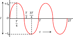
The variation of alternating current with time is shown in figure.

Similarly, sinusoidal voltage of an alternating current source is given by –

$V = V_0 \sin ( \omega t )$ …….. (2)

Here, $( V_0 )$ has the similar nomenclature as that of current. it may be – (1) maximum value or Peak value of alternating voltage or (2) amplitude of alternating voltage.

Average value of an AC Current?

Mean or average value of alternating current is defined as that value of steady current which sends the same amount of charge through a circuit in certain time interval as is sent by an alternating current through the same circuit in half cycle.

Average value or mean value of an AC over half cycle is found to be $( 63.7 \ \% )$ of its peak value $( I_0 )$ .

Therefore, $\quad I_{av} = 0.637 ( I_0 )$

Let, an alternating current is represented by $( I = I_0 \sin ( \omega t ) )$

From definition of electric current, we have –

$I = \left ( \frac {dq}{dt} \right )$

Or, $\quad dq = I dt$

Charge sent by AC in half cycle

The charge sent by the alternating current $( I )$ in time $( dt )$ will be –

$dq = I_0 \sin ( \omega t ) dt$

Therefore, the charge sent by AC in the first half cycle i.e. from $( t = 0 )$ to $\left ( t = \frac {T}{2} \right )$ will be –

$\int dq = \int\limits_{0}^{\frac {T}{2}} I_0 \sin ( \omega t ) dt$

So, $\quad q = I_0 \int\limits_{0}^{\frac {T}{2}} \sin ( \omega t ) dt$

$= I_0 \left [ \frac {- \cos ( \omega t )}{\omega} \right ]_{0}^{\frac {T}{2}}$

$= - \frac {I_0}{\omega} \left [ \cos ( \omega t ) \right ]_{0}^{\frac {T}{2}}$

$= - \frac {I_0}{2 \pi / T} \left [ \cos \left ( \frac {2 \pi}{T} \right ) t \right ]_{0}^{\frac {T}{2}}$

Since, $\quad \omega = \left ( \frac {2 \pi}{T} \right )$

So, $\quad q = - \frac {I_0 T}{2 \pi} \left [ \cos \left ( \frac {2 \pi}{T} \times \frac {T}{2} \right ) - \cos 0 \right ]$

$= - \frac {I_0 T}{2 \pi} \left [ \cos \pi - \cos 0 \right ]$

$= - \frac {I_0 T}{2 \pi} \left [ - 1 - 1 \right ]$

$= \left ( \frac {I_0 T}{\pi} \right )$ …… (1)

Charge sent by Average value of AC in half cycle

Let, $( I_{av} )$ is the mean or average value of AC over positive half cycle, then the charge sent by it in time $\left ( \frac {T}{2} \right )$ will be –

$q = I_{av} \times \left ( \frac {T}{2} \right )$ …… (2)

Therefore, as per definition of mean or average value of current, we have –

$\text {Charge sent by AC in half cycle} = \text {Charge sent by average value of AC in half cycle}$

Therefore, equation (1) and equation (2) must be equal.

Therefore, $\quad I_{av} \times \left ( \frac {T}{2} \right ) = \left ( \frac {I_0 T}{\pi} \right )$

So, $\quad I_{av} = \left ( \frac {2 I_0}{\pi} \right ) = 0.637 \ I_0$

Also, $\quad V_{av} = \left ( \frac {2 V_0}{\pi} \right ) = 0.637 \ V_0$

TO BE NOTED –

The mean or average value of alternating current or voltage over a complete cycle becomes zero.
Hence, ordinary DC instruments like Ammeter and Voltmeter cannot measure AC current or voltage. In AC supply they will give zero reading.

RMS value of an AC Current

Root Mean Square value of alternating current is defined as that steady current which produces the same amount of heat in a conductor in a certain time interval as is produced by the AC in the same conductor during the time period of full cycle i.e. $( T )$ .

Root Mean Square value of alternating current is also known as effective value or virtual value.

Let, an alternating current flows through a conductor of resistance $( R )$ for time $( dt )$ .

Then, heat produced in the conductor will be –

$dH = I^2 R dt$

$= [ I_0 \sin ( \omega t )]^2 R dt$

$= I_0^2 R \sin^2 ( \omega t ) dt$

Heat produced by an AC in one cycle

When AC current flows for time period from $( t = 0 )$ to $( t = T )$ , the heat produced will be –

$\int dH = \int\limits_{0}^{T} I_0^2 R \sin^2 ( \omega t ) dt$

So, $\quad H = I_0^2 R \int\limits_{0}^{T} \sin^2 ( \omega t ) dt$

From trigonometric relations we get –

$\sin^2 \theta = \left [ \frac {1 - \cos ( 2\theta )}{2} \right ]$

Therefore, $\quad H = I_0^2 R \int\limits_{0}^{T} \left [ \frac { 1 - \cos ( 2 \omega t )}{2} \right ] dt$

$= \left ( \frac {I_0^2 R}{2} \right ) \int\limits_{0}^{T} \left [ 1 - \cos ( 2 \omega t ) \right ] dt$

$= \left ( \frac {I_0^2 R}{2} \right ) \left [ \int\limits_{0}^{T} dt - \int\limits_{0}^{T} \cos ( 2 \omega t ) dt \right ]$

$= \left ( \frac {I_0^2 R}{2} \right ) \left [ \left [ t \right ]_{0}^{T} - \left [ \frac {\sin ( 2 \omega t )}{2 \omega} \right ]_{0}^{T} \right ]$

$= \left ( \frac {I_0^2 R}{2} \right ) \left [ \left ( T - 0 \right ) - \frac {1}{2 \omega} \left [ \sin \left ( 2 \times \frac {2 \pi}{T} t \right ) \right ]_{0}^{T} \right ]$

$= \left ( \frac {I_0^2 R}{2} \right ) \left [ T - \frac {1}{2 \omega} \left [ \sin \left ( 2 \times \frac {2 \pi}{T} \times T \right ) - \sin 0 \right ) \right ]$

$= \left ( \frac {I_0^2 R}{2} \right ) \left [ T - \frac {1}{2 \omega} \left ( \sin 4 \pi - \sin 0 \right ) \right ]$

$= \frac {I_0^2 R}{2} \left [ T - \frac {1}{2 \omega} \left ( 0 - 0 \right ) \right ]$

Therefore, $\quad H = \left ( \frac {I_0^2 R}{2} \right ) T$ ……. (1)

Heat produced by RMS value of AC in one cycle

Let, $RMS$ value of an AC current is $( I_{rms} )$ which flows through the conductor. Then –

$H = ( I_{rms} )^2 R T$ ……. (2)

Therefore, as per definition of RMS value of current, we have –

$\text {Heat produced by AC in one cycle} = \text {Heat produced by RMS value of AC in one cycle}$

Therefore, equation (1) and equation (2) must be equal.

Hence, $\quad ( I_{rms} )^2 RT = \left ( \frac {I_0^2 RT}{2} \right )$

So, $\quad I_{rms} = \left ( \frac {I_0}{\sqrt {2}} \right ) = 0.707 \ I_0$

Also, $\quad V_{rms} = \left ( \frac {V_0}{\sqrt {2}} \right ) = 0.707 \ V_0$

AC phasor diagram

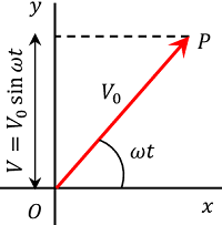
Phasor is a rotating vector which represents a quantity which is varying sinusoidal with time.

An AC phasor is considered as rotating in anticlockwise direction with an angular speed $( \omega )$ .

Instantaneous voltage of AC source is given by –

$V = V_0 \sin ( \omega t )$

So, an alternating current or voltage can be represented in phasor diagram as shown in figure.

In phasor diagram, length of phasor i.e. $( V )$ is proportional to $( V_0 )$ and it describes an angle $( \theta )$ in time $( t )$ , where $( \theta = \omega t )$ and $( \omega )$ is the angular frequency of the voltage of A.C source.

The vertical component of phasor i.e. $[ V = V_0 \sin ( \omega t ) ]$ represents the instantaneous value of the quantity varying sinusoidal.