What are different speeds of molecules?
Molecules of a gas are assumed as rigid and elastic spheres. In a given mass of gas, these molecules remains in constant movement throughout the space available. During the random motion of molecules, they collide with one another and also with the walls of the container. As such the speed of molecules is continuously changing. This fact brings the necessity of three different concepts for speed of gas molecules.
Three types of speed of molecules of gases are very important for thermodynamic point of view. These are –
- Average speed.
- Root mean square speed.
- Most probable speed.
These are explained as below –
1.Average Speed of Molecules
Average speed of molecules is defined as the arithmetic mean of the speeds of the molecules of a gas at a given temperature.
If v_1, \ v_2, \ v_3 \ ..... \ v_n are the speeds of ( n ) molecules of a gas, then the average speed is given by –
\bar {v} = \left ( \frac {v_1 + v_2 + v_3 + ..... + v_n}{n} \right )
Following the Maxwellian speed distribution curve explained below, it can be seen that –
\bar {v} = \sqrt {\frac {8k_BT}{\pi m}} = \sqrt {\frac {8RT}{\pi M}} = \sqrt {\frac {8 PV}{\pi M}}
Where ( m ) is the mass of one molecule and ( M ) is the molecular mass of gas.
2.Root Mean Square speed of Molecules
Root mean square speed of molecules is defined as the square root of mean of the squares of the speeds of the molecules of a gas at a given temperature.
If v_1, \ v_2, \ v_3 \ ..... \ v_n are the speeds of the ( n ) gas molecules, then the root mean square speed is given by –
v_{rms} = \sqrt {\frac {v^2_1 + v^2_2 + v^2_3 + ..... + v^2_n}{n}}
Following the Maxwellian speed distribution curve, it can be seen that –
v_{rms} = \sqrt {\frac {3k_BT}{m}} = \sqrt {\frac {3RT}{M}} = \sqrt {\frac {3 PV}{M}}
Where ( m ) is the mass of a single molecule and ( M ) is the molecular mass of gas.
Therefore, \quad v_{rms} \propto \sqrt T
Thus the root mean square speed is directly proportional to the square root of absolute temperature of the gas.
3.Most Probable speed of Molecules
Most probable speed of molecules is defined as the speed possessed by the maximum number of molecules of a gas sample at a given temperature.
Following the Maxwellian speed distribution curve, it can be seen that –
v_{mp} = \sqrt {\frac {2k_BT}{m}} = \sqrt {\frac {2RT}{M}} = \sqrt {\frac {2 PV}{M}}
Where ( m ) is the mass of a single molecule and ( M ) is the molecular mass of gas.
Maxwell’s Speed Distribution
In gas system molecules randomly collide with each other and also with the walls of the container. So the velocity of a gas molecule remains changing continuously. It may vary over a wide range. However in steady state, the velocity distribution remains fixed in a given mass of gas.
The most probable distribution of speeds of molecules was mathematically derived by Clerk Maxwell.
Consider about following parameters of a sample of gas. Let –
- ( N ) is the total number of gas molecules in given sample of gas.
- ( d N_v ) represents total number of gas molecules having speed in the range between ( v ) and ( v + dv )
- ( n_v ) represents total number of gas molecules having speed ( v )
- ( a ) is a constant whose value is given by \left ( a = \sqrt {\frac {m}{2 \pi k_B T}} \right )
- ( b ) is another constant given by \left ( b = \frac {m}{2 k_B T} \right )
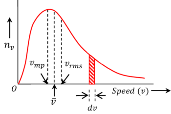
The graph of ( n_v ) versus ( v ) is known as Maxwellian speed distribution and is shown in figure.
Maxwell’s law of speed distribution for gas molecules at temperature ( T ) gives a relation for molecular speeds. This is given by –
d N_v = 4 \ \pi \ N \ a^3 \ e^{-b \ v^2} \ v^2 dv = n_v dv
Features of Maxwellian’s Curve
The important features of the speed distribution curve are explained as follows :
- At a given temperature the speed of molecules can vary from zero to infinity.
- Total area under the curve gives the total number of molecules \left ( N \right ) in the given sample of gas.
- Area of the shaded region gives the number of gas molecules having speed between ( v ) and ( v + dv ) .
- The speed possessed by the largest number of molecules is called most probable speed \left ( v_{mp} \right )
- The curve is not symmetrical about the most probable speed given by \left ( v_{mp} \right ) . Area at the right side of this line is greater than that of the left side. This means that more than ( 50 \% ) of gas molecules have velocity less than \left ( v_{mp} \right )
- Number of gas molecules ( n_v ) corresponding to the root mean square speed \left ( v_{rms} \right ) is less than that of \left ( v_{mp} \right )
- Number of gas molecules having average speed \left ( \bar {v} \right ) is less than \left ( v_{mp} \right ) but more than \left ( v_{rms} \right )
- The minimum speed of molecules towards left of curve is zero whereas at the right of curve there is no limit of minimum speed that a molecule can have.
Relation between Molecular speeds
Following the Maxwellian speed distribution curve, it can be concluded that –
\bar {v} = \sqrt {\frac {8 k_B T}{\pi m}} = \sqrt {\frac {8}{3 \pi}} v_{rms} = 0.92 v_{rms}
Again, \quad v_{mp} = \sqrt {\frac {2k_BT}{m}} = \sqrt {\frac {2}{3}} v_{rms} = 0.816 v_{rms}
Also, \quad v_{rms} = \sqrt {3} \sqrt {\frac {k_B T}{m}} = 1.73 \sqrt {\frac {k_B T}{m}}
Therefore, ratio \quad ( v_{rms} \ : \ \bar {v} \ : \ v_{mp} ) = ( v_{rms} \ : \ 0.92 v_{rms} \ : \ 0.816 v_{rms} )
Or, \quad ( v_{rms} \ : \ \bar {v} \ : \ v_{mp} ) = ( 1 \ : \ 0.92 \ : \ 0.816 )
So, \quad ( v_{rms} \ : \ \bar {v} \ : \ v_{mp} ) = ( 1.73 \ : \ 1.60 \ : \ 1.41 )
Hence, \quad ( v_{rms} ) > ( \bar {v} ) > ( v_{mp} )
Mean Free Path
The molecules of a gas are in a state of continuous, rapid and random motion. The moving molecules frequently collide with one another and also with the walls of the container. Between two collisions, molecules move in a straight line but as they collide their path changes. Hence, each molecule follows a zig-zag path. Between two successive collisions a molecule moves freely with uniform speed.
The mean free path of a gas molecule is defined as the average distance traveled by the molecule between two successive collisions.
If, \lambda_1, \ \lambda_2, \ \lambda_3 ..... etc. are free paths moved by a particular molecule between successive collisions, then its mean free path will be –
\bar {\lambda} = \left ( \frac {\lambda_1 + \ \lambda_2 + \ \lambda_3 + ..... }{\text {Total number of collisions}} \right )
For one mole of a gas, the value of mean free path is given by –
\bar {\lambda} = \left ( \frac {k_B T}{\sqrt {2} d^2 P} \right )
Brownian Motion
Any particle suspended in a fluid is continuously bombarded by the fluid molecules from all directions. The impact of fluid molecules on the particle give raise to an unbalanced force in a certain direction. Thus the particle moves in that direction. As soon as the particle moves a little in that direction, the magnitude and direction of unbalanced force changes due to more impact by the fluid molecules. This makes the particle to move in a new direction. The suspended particle thus moves in a zig-zag manner and tumbles about randomly.
This irregular motion of suspended particles is called Brownian motion.
EXAMPLE –
Pollen grains of a flower suspended in water continuously move in a zig-zag random motion.
Factors affecting Brownian motion
Different factors affecting the Brownian motion are –
- Brownian motion increase with increase in size of suspended particles.
- It increase with increase in temperature of the fluid.
- Brownian motion decrease with decrease in fluid density.
- It decreases with decrease in viscosity of the fluid.