What is Hooke’s Law?
By experiments on behavior of a metal wire under an axial pulling force, an English physicist “Robert Hooke” (1635-1703 A.D.), formulated a law which is popularly known as Hooke’s law. Hooke’s law states that –
The elongation produced in a wire under axial pull is directly proportional to the applied pull.
Hooke’s Law and Young’s theory
Later, another scientist, “Thomas Young” stated that –
Strain produced in the wire is directly proportional to the stress developed in the wire.
Therefore, Young explained about the limitations of Hooke’s law. He modified the Hooke’s law to the more general form as follows –
- Materials show elastic property only up to a certain limit of developed stress. Beyond this limit permanent deformation set up in the material body.
- The maximum stress within which a material body regains its original size and shape after the removal of deforming force, is called elastic limit.
- Within elastic limit, elongation per unit length i.e. strain produced in a wire is directly proportional to the applied pull per unit cross sectional area i.e. stress.
Therefore, within elastic limit –
\text {Stress} \ \propto \ \text {Strain}
So, \quad \left ( \frac {\text {Stress}}{\text {Strain}} \right ) = \text {Constant}
This constant of proportionality is called modulus of elasticity or coefficient of elasticity of the material.
Load – Extension Curve
Robert Hooke use a device called “Extensometer” to do his experiment for measuring the extension of a wire under a tensile load.
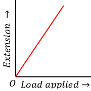
Consider about the elastic curve of an ductile material as shown in figure. In this experiment, a wire made of an elastic material is hanged in the device and loaded under the axial tensile load. The load is gradually increases and the extensions in the wire are recorded for each loading.
The values of applied tensile load are plotted along X axis and the resulted elongation is plotted along Y axis. The obtained curve is called “Load – Extension Curve”.
Hooke noted that, when the applied load is within certain limit, the obtained curve is a straight line passing through the origin. So, the extension in the length of wire is proportional to the load applied.
This represents the correctness of Hooke’s law.
Stress
If a body gets deformed under the action of an external force, then at each section of the body an internal restoring force of reaction is set up which tends to restore the body into its original state.
The internal restoring force set up in the deformed body per unit area of cross-section is called stress.
The restoring force is equal but opposite to the external deforming force. Therefore, stress is expressed as –
\text {Stress} = \frac {\text {Applied force}}{\text {Area}}
The SI unit of stress is ( \text {N-m}^{-2} ) and the CGS unit is ( \text {dyne-cm}^{-2} ) .
Types of Stress
Different types of stresses developed in a deformed body are –
Longitudinal Stress
It is defined as the restoring force set up per unit cross-sectional area of a body when the length of the body changes in the direction of the deforming force.
If ( F_{axial} ) is the applied external force on a rigid body having area of cross section ( A )
Then, longitudinal stress is given by –
f = \left ( \frac {F_{axial}}{A} \right )
Longitudinal stress is of two types –
- Tensile stress – It is the restoring force set up per unit cross-sectional area of a body when its length increases under a deforming force.
- Compressive stress – It is the restoring force set up per unit cross-sectional area of a body when its length decreases under a deforming force.
Tangential or Shearing Stress
When a deforming force acts tangentially to the surface of a body, it produces a change in the shape of the body.
If ( F_{tangential} ) is the applied external force on a rigid body tangentially over a surface area ( A )
Then, shearing stress is given by –
f = \left ( \frac {F_{tangential}}{A} \right )
Strain
The ratio of the change produced in any dimension of a rigid body to the original dimension is called strain.
Therefore, strain is given by –
Strain = \left ( \frac {\text {Change in dimension}}{\text {Original dimension}} \right )
Since, strain is a ratio of two similar quantities, so it is dimensionless and has no units.
Types of Strain
Different types of strain developed in a body are –
Longitudinal Strain
It is defined as the ratio of increase or decrease in length and original length.
Therefore, \quad \text {Longitudinal strain} = \left ( \frac {\text {Change in length}}{\text {Original length}} \right ) = \left ( \frac {\Delta l}{l} \right )
Volumetric Strain
It is defined as the ratio of change in volume and original volume.
Therefore, \quad \text {Volumetric strain} = \left ( \frac {\text {Change in volume}}{\text {Original volume}} \right ) = \left ( \frac {\Delta V}{V} \right )
Shear Strain
It is defined as the tangent of the angle θ (in radian), through which a face of body which was originally perpendicular to the fixed surface gets deformed.
Therefore, \quad \text {Shear strain} = \tan \theta = \left ( \frac {\text {Relative distance between two parallel planes}}{\text {Distance between parallel planes}} \right )
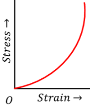
Stress – Strain curve & Hooke’s Law
Consider about the following figure. The figure shows a typical strain – strain curve relating to Hooke’s law of a ductile metal wire which is loaded by a gradually increasing axial load. This curve is also known as elastic curve.
It has six distinct regions as shown in figure.
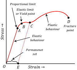
(1) REGION OA –
The initial part OA of the graph is a straight line indicating that stress is proportional to strain. Upto the point A , Hooke’s law is obeyed. The point A is called the proportional limit. In this region the wire is perfectly elastic.
(2) REGION AB –
After the point A , the stress is not proportional to the strain. However, if the external load is removed at any point between O and B , the curve is retraced along BAO and the wire attains its original length.
The portion OB of the graph is called elastic region and the point B is called elastic limit or yield point. The stress corresponding to the yield point is called yield strength ( S_y )
Up to the point B , the elastic forces of the material are conservative forces i.e. when the load is removed and the material returns to its original size, then the work done in producing the deformation is completely recovered.
(3) REGION BC –
Beyond the point B , the strain increases more rapidly than stress. If the load is removed at any point C , the wire does not return to its original length but it traces dashed line CE . Even on reducing the stress to zero, a residual strain equal to OE is left in the wire. Thus the material is said to have acquired a permanent set.
The fact that the stress-strain curve is not retraced on reversing the strain is called elastic hysteresis.
(4) REGION CD –
If the load is increased beyond the point C , there is a large increase in the strain i.e. the length of the wire increases tremendously. In this region a neck is develop at some point D of the wire and the wire ultimately breaks at this point. The point D is called the fracture point.
(5) REGION OB –
In the region from O to B , the material regains its original shape and size upon removal of external applied load. Hence this region is called elastic region of the curve.
(6) REGION BD –
In the region between B and D , the material gets permanent deformation. This region is called plastic region and the material is said to undergo plastic flow or plastic deformation.
The stress corresponding to the breaking point D is called ultimate strength or tensile strength of the material.
Types of materials based on elastic curve
On the basis of strain – strain curve, materials are classified into following types –
Ductile material
Materials which have large plastic range i.e. region between B and D of strain – strain curve, are called ductile materials.
As shown in the stress-strain curve, the fracture point is widely separated from the elastic limit point B . Such materials undergo an irreversible increase in length before breaking takes place at point D . So, these materials can be drawn into thin wires.
Example –
Copper, Silver, Iron, Steel, Aluminium, etc.
The property by which any material can be drawn into thin wires by the application of tensile load is called ductility.
Brittle material
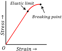
The materials which have very small plastic range i.e. short region between B to D of strain – strain curve are called brittle materials. Such materials break as soon as the stress is increased beyond the elastic limit. Their breaking point D lies just close to their elastic limit point B as shown in figure.
Example –
Cast iron, Glass, Ceramics, etc.
The property by which any material breaks or fail to withstand as soon as the the stress increases above the elastic limit is called brittleness.
Malleable material
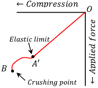
Stress – strain behavior of solid materials are different in case of tensile load and compressive load. Some materials show good plastic behavior under the action of compressive load.
When a material is compressed, a stage is reached beyond which it cannot recover its original shape after the deforming force is removed. This is called the elastic limit point A' for compression as shown in figure. The solid then behaves like a plastic body. The yield point B' obtained under compression is called crushing point.
Between the points A' and B' , metals are said to be malleable i.e., they can be hammered or rolled into thin sheets.
Example –
Gold, Silver, Lead etc.
The property by which any material can be hammered and flattened into thin sheets under the action of compressive load is called malleability.
Elastomers
The materials which can be elastically stretched to a large values of strain are called elastomers. These materials has a large range of elastic region but no well defined plastic region.
Elastomers do not obey Hooke’s law. Their Young’s modulus is also very small.
Example –
- Rubber can be stretched to several times of its original length but still it can regain its original length when the applied force is removed. It just breaks when pulled beyond a certain limit.
- In our body, the elastic tissue of aorta is an elastomer.
See numerical problems based on this article.